A Versatile and Inexpensive Technique for Measuring Color of Foods

A frequent challenge in conducting research is to find the right tools with a limited budget. We recently encountered this challenge when searching for a versatile and inexpensive technique to measure the color of the bottom surface of microwaved pizza.

Specifically, we needed to measure the color profile at various locations on the surface and to store the images of food samples for future use. Although our department has a HunterLab Colorimeter and a Minolta Chroma Meter, these instruments did not meet our needs because they can provide only a single average measurement for each food sample—it would be too time-consuming if these instruments were used to obtain point-by-point measurements at many locations on the food sample for constructing the color profile. We found several commercial color-measuring instruments via the Internet, but these instruments were beyond our budget and were more suitable for quality control than research purposes. 

Fortunately, we knew that Adobe Photoshop software had the capability to analyze digital images for color. We thought that perhaps we could develop a technique using the software and a digital camera to meet our needs. Consequently, we developed the technique and were delighted with the results. Since other food scientists and technologists could benefit from our experience, we wrote this article to share our technique and illustrate its application. 

Color Measurement Technique
Our technique involves setting up a lighting system, using a high-resolution digital camera to capture images of food samples, and using Photoshop software to obtain color parameters. A computer (Pentium III, 64 MB RAM, 20 GB hard disk or higher recommended) is also needed to run the software. Excluding the computer, the combined cost of the lighting system, digital camera, and software is under $1,500.

Color Model. In defining and displaying color, it is necessary to select a color model. Photoshop can display color in three different models: RGB (red, green, blue), CMYK (cyan, magenta, yellow, black), and L*a*b*. RGB is used for displaying colors on computer monitors, CMYK is used for defining process ink colors in printing, and L*a*b* is commonly used in measuring colors in food research. 

L*a*b* is an international standard for color measurements, adopted by the Commission Internationale d’ Eclairage (CIE) in 1976. This color model is designed to be device independent, creating consistent color regardless of the device (such as monitor, printer, or scanner) used to create or output the image. L* is the luminance or lightness component, which ranges from 0 to 100, and a* (from green to red) and b* (from blue to yellow) are the two chromatic components, which range from –120 to +120 (Anonymous, 1998). The principles of color measurements can be found elsewhere, and there are other color models used in food research (Hunt, 1991; Francis and Clydesdale, 1975; Clydesdale, 1978).

Lighting System. It is important to use the proper light source, since the color of the food sample depends on the part of the spectrum reflected from it (Francis and Clydesdale, 1975). The light source is specified by its color temperature, and the standard light sources (defined by CIE) commonly used in food research are A (2,856 K), C (6,774 K), D₆₅ (6,500 K), and D (7,500 K). The latter three light sources are designed to mimic variations of daylight (Lawless and Heymann, 1998). 

--- PAGE BREAK ---

The angle between the camera lens axis and the lighting source axis should be around 45°. This is because in color measurements we are interested in capturing the diffuse reflection responsible for the color, which occurs at 45° from the incident light (Francis and Clydesdale, 1975). 

The light intensity over the food sample should be uniform. This can be achieved through experimenting with various lighting arrangements (such as varying the distance between the light source and the food sample, taking the pictures in a dark room), and checking the results with a light meter.

Digital Camera. A digital camera records images on an electric light sensor that is made up of millions of tiny points called pixels. Two major factors that affect the quality of the image are resolution and file compression. Resolution is related to the number of pixels on the light sensor: the more pixels, the higher the resolution and the higher the image quality. File compression reduces the amount of memory taken up by the image and allows more images to be stored. The trade-off for compressing the file is loss of image quality. 

We recommend that the camera have a minimum resolution of 1,600 x 1,200 pixels and the capability of storing digital images as a TIFF file (non-compressed file). We also recommend that the camera have macro and zoom features, a remote control, and a memory card of at least 32 Mb. Color standards (such as the Munsell color standards) should be photographed and analyzed periodically to ensure that the lighting system and the camera are working properly.

Software. Photoshop (Adobe Systems Inc., San Jose, Calif.) is a software program used by graphics producers and photographers for photo retouching and image editing. We also find several features in the software that are particularly useful to obtain color parameters for digital images of food samples:
As mentioned above, the software can display color in L*a*b*, the preferred color model for food research. 

It also has selection tools (such as the Elliptical Marquee and the Rectangular Marquee) for selecting any part of the image, and the dimensions of the selection can be conveniently displayed. Once a selection is made, the Histogram Window of the software provides the parameter values for Lightness, a, and b. For each of these three parameters, graphs of cumulative distribution, mean, standard deviation, median, and number of pixels for the selection can also be displayed. The software uses 256 levels, ranging from 0 to 255, to characterize Lightness, a, and b values of the pixels. To convert Lightness, a, and b values obtained from the Histogram Window to L*, a*, and b*, the following formulas can be used: 

L* = (Lightness/250)(100)        (1)

a* = (240a/255) – 120              (2)

b* = (240b/255) – 120              (3)

Another useful selection tool is the Magic Wand Tool. By positioning it on any pixel in an image, one not only can obtain the L*, a*, and b* values of that pixel, but also can select from the whole image all the pixels that are quite similar in color to the particular pixel. The range of L*, a*, and b* values of the pixels thus selected is controlled by the tolerance value of the Magic Wand Tool. 

--- PAGE BREAK ---

Color Profile of Microwaved Pizza
 The color of the bottom surface of cooked pizza is not only important to visual perception, but also related to crispness. It is well known that microwave cooking does not produce crisp and browned pizza. A method to overcome this problem is to microwave the pizza in contact with a susceptor, which is usually made of a metallized polyethylene terephthalate (PET) film laminated to paperboard. The susceptor absorbs microwave energy, heats up rapidly to high temperatures, and causes browning of the contacting food surfaces (Buffler, 1993; Zuckerman and Miltz, 1997). The application of our technique to measure and compare the color of microwaved pizza with and without susceptor is illustrated below. 

Commercial ready-to-cook frozen pizzas, 3.5-in radius and 0.6 in thick, of the same brand were used. The pizzas were microwaved either on a plain paperboard or on a susceptor (optical density of 0.28). The microwave oven had a cavity volume of 1.6 cu ft, a turntable, and an 1,100-W power output (measured by the IEC-705 method). The pizzas were microwaved at 100% power for either 3 or 3.5 min. After microwaving, they were cooled to room temperature and then flipped over. 

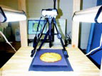
Fig. 1 shows the experimental setup of the lighting system, digital camera, and food sample. The lighting system consisted of two CIE source D₆₅ lamps (Bulb Direct, www.bulbdirect.com), 17.7 in long, mounted on two sides of a frame, on either side of the food sample, 12 in above and at an angle of 45° to the food sample plane. 

The digital camera (Olympus, model C-2000Z) was held securely on a tripod, and the lens faced down toward the food sample. The distance from the bottom of the camera lens to the food sample plane was 12 in. Images of the bottom surface of the pizza were taken under the following camera settings: aperture priority mode with the lens aperture at f11, no flash, daylight conditions, macro mode on, remote mode on, sound on, resolution 1,600 x 1,200 pixels, with the images saved in memory card as TIFF files. 

After zooming the lens (so that the pizza covered the whole field of view) and focusing, the picture was taken with the remote control. The pictures were downloaded to the personal computer via the RS-232C interface, using the software provided with the digital camera. Downloading of each TIFF file (about 5.5 Mb in size) took about 10 min. 

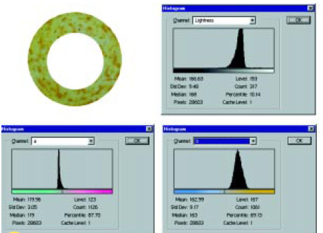
After the picture (Fig. 2) was opened in Photoshop, the Elliptical Marquee Tool (constrained to circular selections by holding down the shift key while dragging the mouse) was used to select the image of the whole pizza, with the dark background omitted. The selected image was copied and pasted to a new file, and the whole pizza was then separated into three sections (Fig. 3). The outer section was created by cutting a circle of 2.5-in radius from the whole pizza, and the middle section was created by cutting a circle of 1.5-in radius (the inner section) from the 2.5-in-radius circle. For convenience, the Fix Size feature in the Marquee Options was also used to select the circles of specific dimensions. To correlate those dimensions to the actual food sample dimensions, a ruler was photographed under the same conditions and the correlation factor was estimated.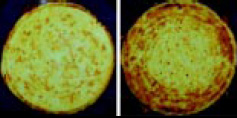 

To obtain L*, a*, b* values of the whole pizza and the three sections, the default RGB mode was changed to Lab Color mode. Each section was selected by first clicking all the white background using the Magic Wand Tool while holding the shift key, then choosing the Inverse Command in the Select Menu. In Fig. 4, the middle section was selected using this technique, and the Histogram Window displayed the mean Lightness, a, and b values, which were then converted to L*, a*, b* using Eqs. 1–3. 

We defined the % dark surface of a selection as: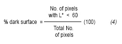 

--- PAGE BREAK ---

The criterion of L* < 60 was chosen here based on our experience with this product, but other criteria could also be chosen, depending on the requirement of the study being undertaken. In Fig. 4, the % dark surface was estimated using Level and Percentile. Level is same as Lightness, which can be converted to L* using Eq. 1. In our case, L* = 60 corresponded to Level = 153, which was selected by moving the pointer of the computer screen, inside and horizontally across the Lightness Chart, until the value of Level changed to 153. The corresponding Percentile was 8.4%, which was the % dark surface with L* < 60. The value of Percentile can also be easily obtained for any range of L* (e.g., a range of 50 < L* <70).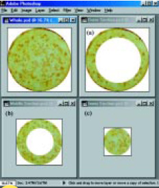 

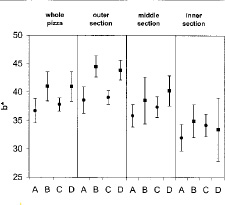
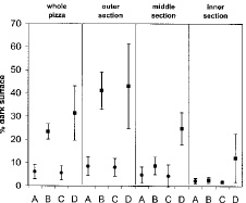
Figs. 5–8 show the values of L*, a*, b* and the % dark surface for the whole pizza and the three sections. Each datum is the average of five replicates, and the error bar represents ± one standard deviation. The mean L* values for pizzas microwaved on the susceptor were higher than those microwaved on plain paperboard. The darkening achieved was more pronounced in the outer section than in the middle section and the inner section because of the edge effect (Buffler, 1993). Increasing the microwaving time from 3 min to 3.5 min decreased the L* values only for the samples microwaved on the susceptor. There were more variations in the samples microwaved on the susceptor, as indicated by the larger error bars. Similar observations can also be made for the a* and b* values and the % dark surface. 

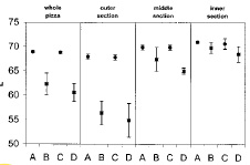
A Versatile System 
We have found this simple technique to be versatile, affordable, and easy to use. It can be applied to many other foods besides pizza. For example, we have used the technique to analyze color for cereal bars. However, like other techniques, food samples with flat surfaces are easier to handle.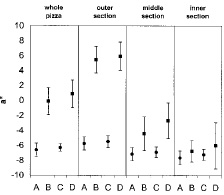 

SPYRIDON E. PAPADAKIS, SITI ABDUL-MALEK, RICKY EMERY KAMDEM, AND KIT L. YAM
Author Papadakis, a Professional Member of IFT, is Professor, Dept. of Food Technology, T.E.I. of Athens, Greece. Authors Malek and Kamdem are Ph.D. students, and author Yam, a Professional Member of IFT, is Associate Professor, Dept. of Food Science, Rutgers University, New Brunswick, NJ 08901. Send reprint requests to author Yam.

Edited by Neil H. Mermelstein
Senior Editor

References

Anonymous. 1998. Adobe Photoshop 5.0 User Guide for Macintosh and Windows. Adobe Systems Inc., San Jose, Calif.
Buffler, C.R. 1993. “Microwave Cooking and Processing: Engineering Fundamentals for the Food Scientist.” Van Nostrand Reinhold, New York.
Clydesdale, F.M. 1978. Colorimetry: Methodology and applications, CRC Crit. Rev. Food Sci. Nutr. 10(3): 243-301.
Francis, F.J. and Clydesdale, F.M. 1975. “Food Colorimetry: Theory and Applications.” Avi Publishing, Westport, Conn.
Hunt, R.W.G. 1991. “Measuring Colour,” 2nd ed. Ellis Horwood, New York.
Zuckerman, H. and Miltz, J. 1997. Prediction of dough browning in the microwave oven from temperatures at susceptor/product interface. Food Sci. Technol. 30: 519-524.